[edit]
1 нҷҳкІҪм„ёнҢ… #
- Rкё°л°ҳ лӢӨліҖлҹү 분м„қ/м •к°•лӘЁ,к№ҖлӘ…к·ј/көҗмҡ°мӮ¬мқҳ мҳҲм ң
 мҳҲм ңм—җ м“°мқҙлҠ” лҚ°мқҙн„°
- Windows Rм—җм„ң [нҢҢмқј] -> [л””л үнҶ лҰ¬ліҖкІҪ] мқ„ м„ нғқн•ҳм—¬ мҳҲм ң лҚ°мқҙн„°к°Җ мһҲлҠ” л””л үнҶ лҰ¬лЎң ліҖкІҪ]
[edit]
2 кіө분мӮ°(Covariance) #
- кіө분мӮ°мқҳ к°Ғ ліҖлҹүм—җ лҢҖн•ң нҺём°Ёмқҳ кіұ
- ліҖмҲҳк°„мқҳ мғҒкҙҖкҙҖкі„лҘј м•Ңм•„ліҙкё° мң„н•ң 분м„қ л°©лІ•, лҳҗ лӢӨлҘё л°©лІ•мңјлЎң мғҒкҙҖ분м„қ(Correlation)мқҙ мһҲлӢӨ.
- кіө분мӮ° > 0 кІҪмҡ°: Xк°’мқҙ м»Өм§Ҳл•Ң Yк°’лҸ„ м»Өм§Җкұ°лӮҳ, Xк°’мқҙ мһ‘м•„м§Ҳ л•Ң Yк°’лҸ„ мһ‘м•„м§ҖлҠ” кІҪмҡ°
- кіө분мӮ° < 0 кІҪмҡ°: Xк°’мқҙ м»Өм§Ҳл•Ң Yк°’мқҖ мһ‘м•„м§Җкұ°лӮҳ, Xк°’мқҙ мһ‘м•„м§Ҳ л•Ң Yк°’мқҖ м»Өм§ҖлҠ” кІҪмҡ°
- кіө분мӮ° = 0 кІҪмҡ°: XмҷҖ Yк°„м—җ к·ңм№ҷм„ұмқҙ м—Ҷкұ°лӮҳ н•ң ліҖмҲҳк°Җ кі м •м Ғмқё к°’мқ„ к°Җм§ҖлҠ” кІҪмҡ°
- мёЎм •лӢЁмң„м—җ л”°лқј к°’мқҙ лӢ¬лқјм§ҖлҜҖлЎң мғҒкҙҖкҙҖкі„мқҳ м •лҸ„лҘј лӮҳнғҖлӮҙкё°м—җлҠ” л¶Җм Ғн•©н•ҳлӢӨ.
- кҙҖкі„мқҳ м •лҸ„лҠ” мғҒкҙҖкі„мҲҳ мӮ¬мҡ©, -1 <= мғҒкҙҖкі„мҲҳ <= 1
- мғҒкҙҖкі„мҲҳ = кіө분мӮ°(X,Y) / н‘ңмӨҖнҺём°Ё(X) * н‘ңмӨҖнҺём°Ё(Y)
[edit]
3 кіө분мӮ°н–үл ¬ #
- л§җк·ёлҢҖлЎң кіө분мӮ°мқҳ н–үл ¬мқҙлӢӨ.
- cov.wt н•ЁмҲҳлҘј мқҙмҡ©
- кІ°кіј
- $cov кіө분мӮ°н–үл ¬
- $center к°Ғ м—ҙмқҳ нҸүк·
- $n.obs н–үмҲҳ
- $cor мғҒкҙҖкі„мҲҳн–үл ¬
- $cov кіө분мӮ°н–үл ¬
> cost.d <-read.table("cost.d", header=T)
> cov.wt(cost.d, cor=T)
$cov
             fuel    repair   capital
fuel    23.013361 12.366395  2.906609
repair  12.366395 17.544111  4.773082
capital  2.906609  4.773082 13.963334

$center
     fuel    repair   capital
12.218611  8.112500  9.590278

$n.obs
[1] 36

$cor
             fuel    repair   capital
fuel    1.0000000 0.6154424 0.1621444
repair  0.6154424 1.0000000 0.3049570
capital 0.1621444 0.3049570 1.0000000

> pairs(cost.d)
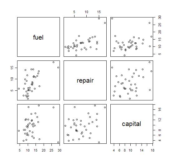
кІ°кіј н•ҙм„қмқ„ н•ҙліҙл©ҙ..
- fule(м—°лЈҢ비), repair(мҲҳлҰ¬л№„), capital(мһҗліёкёҲ)мқҖ лӘЁл‘җ м–‘мқҳ мғҒкҙҖкҙҖкі„лҘј к°Җ진лӢӨ.
- fuleкіј repairмқҳ мғҒкҙҖкі„мҲҳлҠ” 0.62
- fuleкіј capitalмқҳ мғҒкҙҖкі„мҲҳлҠ” 0.16
- repairмҷҖ capitalмқҳ мғҒкҙҖкі„мҲҳлҠ” 0.35
- к·ёлҹ¬лҜҖлЎң fule(м—°лЈҢ비), repair(мҲҳлҰ¬л№„)к°Җ к°ҖмһҘ мғҒкҙҖкҙҖкі„к°Җ лҶ’лӢӨкі ліј мҲҳ мһҲлӢӨ.
- ліҙнҶө мғҒкҙҖкі„мҲҳк°Җ 0.8 мқҙмғҒмқҙм–ҙм•ј мқҳлҜёк°Җ мһҲлӢӨкі ліёлӢӨкі н•ңлӢӨ.
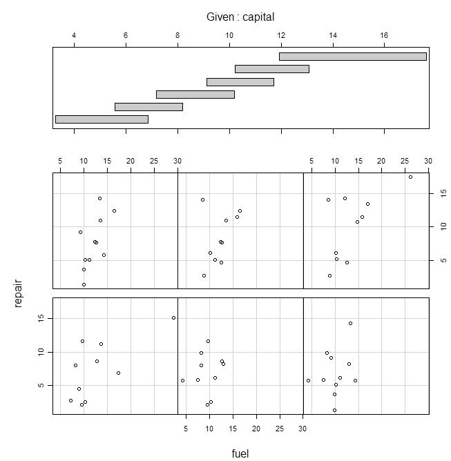
#мЎ°кұҙл¶Җ мӮ°м җлҸ„ #мһҗліёкёҲмқҙ мЎ°кұҙмңјлЎң мЈјм–ҙ진 мғҒнҷ©м—җм„ң м—°лЈҢ비(лҸ…лҰҪліҖмҲҳ)мҷҖ мҲҳлҰ¬л№„(л°ҳмқ‘ліҖмҲҳ)мӮ¬мқҙмқҳ кҙҖкі„ coplot(repair~fuel|capital, data=cost.d)
[edit]
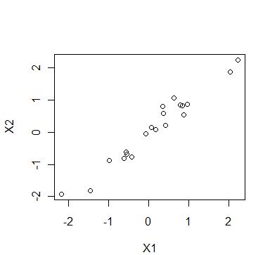
4 мқҙліҖлҹү мһҗлЈҢмқҳ мғҒкҙҖкі„мҲҳлҘј к·ёлһҳн”„лЎң н‘ңнҳ„н•ҳкё° #
лӢӨмқҢмқҖ X1, X2 л‘җ ліҖлҹүмқҳ мғҒкҙҖкі„мҲҳк°Җ 0.98мқё лӮңмҲҳм—җ лҢҖн•ң к·ёлһҳн”„лӢӨ.
> set.seed(2)
> library(mvtnorm)
> x <- rmvnorm(20, sigma=matrix(c(1, 0.98, 0.98, 1), 2))
> x
             [,1]        [,2]
 [1,]  0.62872170  1.05125106
 [2,] -0.61625134 -0.81208810
 [3,]  2.23543105  2.23568460
 [4,]  0.36178518  0.79807392
 [5,] -0.05901189 -0.04696427
 [6,] -1.44903706 -1.81448776
 [7,]  0.85017069  0.81754232
 [8,] -0.56312456 -0.61359221
 [9,]  2.03787185  1.86925931
[10,]  0.07583804  0.13642630
[11,]  0.79101426  0.83645122
[12,]  0.96199934  0.86826634
[13,]  0.37699900  0.58472713
[14,] -0.98481735 -0.87797193
[15,]  0.88841158  0.52652788
[16,] -2.16636324 -1.92376783
[17,] -0.41200937 -0.78035322
[18,] -0.54347793 -0.67618649
[19,]  0.43040268  0.20810378
[20,]  0.17868536  0.08269170
> plot(x[,1], x[,2], xlab="X1", ylab="X2")
[edit]
5 лӢӨмӨ‘мғҒкҙҖкі„мҲҳ #
- лӢӨмӨ‘мғҒкҙҖкі„мҲҳлҠ” н•ҳлӮҳмқҳ ліҖмҲҳк°Җ лӢӨлҘё м—¬лҹ¬ ліҖмҲҳл“Ө(ліҖмҲҳк·ёлЈ№)кіјмқҳ мғҒкҙҖкі„мҲҳлҘј мқҳлҜён•ңлӢӨ. (м„ нҳ•кҙҖкі„)
- 0 <= лӢӨмӨ‘мғҒкҙҖкі„мҲҳ <= 1
- KshirsagarлһҖ мӮ¬лһҢмқҙ 1972л…„м—җ 맹그лҹ¬м„ң мӮ¬лһҢ мЎ°лӮё к·Җм°®кІҢ н•ңлӢӨ.
mcc.f<-function(x, var1, var2)
{
	s<-var(x)
	s0<-sqrt(s[var1,var1])
	s0q<-s[var1,var2]
	Sq<-s[var2,var2]

	sqrt(s0q%*%solve(Sq)%*%s0q)/s0
}
лӢӨмқҢкіј к°ҷмқҙ мң„мқҳ н•ЁмҲҳлҘј мқҙмҡ©н•ҳм—¬ лӢӨмӨ‘мғҒкҙҖкі„мҲҳлҘј кө¬н• мҲҳ мһҲлӢӨ.
cost.d <-read.table("cost.d", header=T)
source("mcc.f")
mcc.f(cost.d, 1, c(2,3))

          [,1]
[1,] 0.6160264
кІ°кіј
- лӢӨмӨ‘мӮ°кҙҖкі„мҲҳлҠ” 0.6160264
- мҰү, fuelкіј (repair, capital)мқҳ мғҒкҙҖкҙҖкі„мқҙлӢӨ.
- solveн•ЁмҲҳлҠ” м—ӯн–үл ¬мқ„ кө¬н•ҳлҠ” н•ЁмҲҳмқҙкі , %*%лҠ” н–үл ¬мқҳ кіұмқҙлӢӨ.
[edit]
6 л¶Җ분мғҒкҙҖкі„мҲҳ #
л‘җ ліҖмҲҳ к·ёлЈ№к°„мқҳ мғҒкҙҖкі„мҲҳлӢӨ. лӢӨмқҢмқҳ мӮ¬мҡ©мһҗ м •мқҳ н•ЁмҲҳлҘј мқҙмҡ©н•ңлӢӨ.
pcc.f<-function(x,z1,z2,x2)
{
	x<-as.matrix(x)
	s<-var(x)
	s22<-s[x2,x2]

	y1<-x[,z1]-x[,x2]%*%solve(s22)%*%s[z1,x2]
	y2<-x[,z2]-x[,x2]%*%solve(s22)%*%s[z2,x2]
	cor(y1,y2)
}
soil.d <-read.table("soil.d", header=T)
source("pcc.f")
pcc.f(soil.d, 1, 2, c(3,4))

          [,1]
[1,] 0.7475448
кІ°кіјлҠ” 0.748мқҙлӢӨ. soil.dлҠ” нҶ м–‘м„ұ분мһҗлЈҢлқјкі н•ңлӢӨ.
[edit]
7 н‘ёлҰ¬м—җ кёүмҲҳмқҳ н‘ңнҳ„(м•Өл“ңлҘҳмҠӨ к·ёлҰј) #
мқҙл ҮкІҢ мҚЁлЁ№лҠ”лӢӨ.
- лӢӨлҘё мһҗлЈҢмҷҖ нҒ° м°ЁмқҙлҘј лӮҳнғҖлӮҙлҠ” мқҙмғҒм№ҳлҘј л°ңкІ¬
- мһҗлЈҢк°„мқҳ кұ°лҰ¬ мң м§Җ
- мһҗлЈҢмқҳ к·ёлЈ№нҷ”
#м•Өл“ңлҘҳмҠӨмқҳ к·ёлҰј(н‘ёлҰ¬м—җ кёүмҲҳ, мһҗлЈҢк°„мқҳ кұ°лҰ¬лҘј кұ°лҰ¬лҘј мң м§Җн•ҳлҠ” мқҙмң )
andrews.f<-function(x,v)
{
n<-nrow(x)
p<-ncol(x)
nv<-length(v)
x<-as.matrix(x)
m<-cov.wt(x)$center
M<-matrix(m*rep(1,n*p),n,p,byrow=T)
d<-diag(1/sqrt(diag(cov.wt(x)$cov)))
x<-(x-M)%*%d
l<-100
tt<-seq(from=-pi,to=pi,length=l);
andr.v<-c(rep(1/sqrt(2),l))
for(i in 1:((p-1)/2))
andr.v<-c(andr.v,sin(i*tt),cos(i*tt))
if( p%%2 == 0 )
andr.v<-andr.v[-( ((p-1)*l+1): p*l )]
andr.m<-matrix(andr.v,nrow=l,ncol=p)
y <- andr.m%*%t(x)
z <- matrix(0,nv*l,2)
lab<-vector("numeric",nv*l)
plot(rep(tt,n),as.vector(y),type="n",xlab="t",ylab="Andrews plot")
for(i in 1:nv) {
lines(tt,y[,v[i]])
for(j in 1:l ) {
z[(i-1)*l+j,1]<-tt[j]
z[(i-1)*l+j,2]<-y[j,v[i]]
lab[(i-1)*l+j]<-v[i]
}
}
abline(h=0)
identify(z,labels=lab)
}
andrews.f(cost.d, c(1:36))
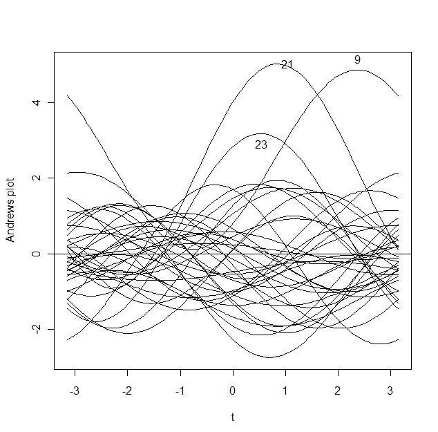
к·ёлҰјм—җм„ң к°ҖмһҘ ліјлЎқн•ҳкІҢ мҳ¬лқјмҳЁ кіЎм„ м—җ л§Ҳмҡ°мҠӨлҘј нҒҙлҰӯн•ҳл©ҙ к°’мқҙ лӮҳнғҖлӮңлӢӨ. 9, 21мқҖ лӢӨлҘё мһҗлЈҢмҷҖ нҒ° м°ЁмқҙлҘј ліҙмқҙлҜҖлЎң к°ҖлҠҘм„ұмқҙ мһҲлӢӨ. м•Өл“ңлҘҳмҠӨ к·ёлҰјмқҖ 9, 21, 23мқҙл©ҙ 충분н•ҳлӢӨ.
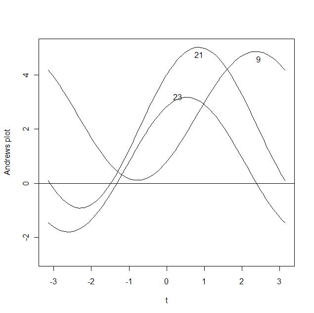
andrews.f(cost.d, c(9, 21, 23))
п»ҝ